Plotting in {EGAnet} has become much more flexible by passing on
most arguments to {GGally}’s ggnet2 (some arguments might
not change to keep a consistent {EGAnet} style to the plots). This Wiki
walks through some of the flexibility available in {EGAnet}’s plots.
This demonstration is only the start – you can use these plots as the
foundation for your own creations. These examples focus solely on
EGA plotting but apply to all *EGA plots.
The sections below start with the basics — getting a plot on screen
and tweaking the obvious things (color, size, labels) — then move into
more advanced usage that leans on how {EGAnet} builds its plots on top
of ggnet2 internally: reusing a layout across plots, sizing
nodes correctly by community, and a couple of genuine gotchas worth
knowing about before you hit them.
Quick Reference
A cheat sheet for the elements people change most often — every
argument below goes directly into plot():
| Want to change… | Argument(s) | Example | See |
|---|---|---|---|
| Node colors | color.palette, node.color |
plot(x, color.palette = "blue.ridge2") |
Nodes |
| Node size | node.size |
plot(x, node.size = 12) |
Nodes |
| Node transparency | node.alpha |
plot(x, node.alpha = 0.5) |
Nodes |
| Node shape | node.shape (or shape) |
plot(x, node.shape = 17) |
Nodes |
| Node/item labels | node.label, label.size,
label.color |
plot(x, node.label = paste0("Item ", 1:18)) |
Labels |
| Node layout/arrangement | layout (or mode) |
plot(x, layout = "circle") |
Layout |
| Edge color | edge.color |
plot(x, edge.color = c("pink", "black")) |
Edges |
| Edge width | edge.size |
plot(x, edge.size = 12) |
Edges |
| Edge transparency | edge.alpha |
plot(x, edge.alpha = 0.1) |
Edges |
| Edge line type | edge.lty |
plot(x, edge.lty = c("dashed", "solid")) |
Edges |
| Edge value labels | edge.label |
plot(x, edge.label = edge_values) |
Edge Value Labels |
| Legend text | legend.names, legend.title |
plot(x, legend.names = c("Dim 1", "Dim 2")) |
Legend |
| Legend position/size | legend.position, legend.size |
plot(x, legend.position = "bottom") |
Legend Position and Size |
| Plot title | title, or + ggtitle(...) |
plot(x, title = "My Title") |
Title |
| Panel layout (multi-network plots) | ncol, nrow, legend,
common.legend |
compare.EGA.plots(x, y, ncol = 1) |
Controlling Panel Layout of Composite Plots |
| Themes, annotations, zoom, selective legends | any {ggplot2} layer |
plot(x) + theme_minimal() |
Combining with ggplot2 |
Basic
Basic Plot
# Load necessary packages
library(EGAnet); library(GGally); library(ggplot2)

# Estimate EGA
ega.wmt <- EGA(wmt2[,7:24], plot.EGA = FALSE)

# Plot
plot(ega.wmt)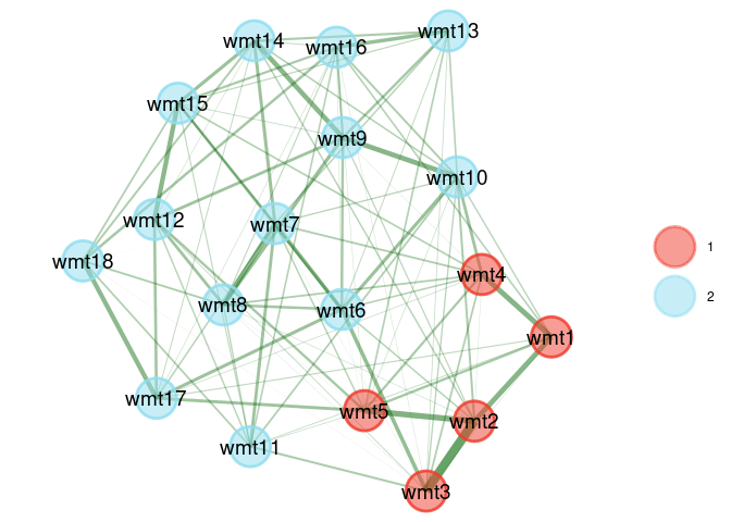
Shortcut Names
The rest of this page mostly uses ggnet2’s own argument
names (node.color, node.alpha, and so on),
since they’re unambiguous. But {EGAnet} also accepts five shorter,
friendlier names for the ones people reach for most — each is completely
interchangeable with its real argument, so use whichever reads better in
your own code:
| Shortcut | Real argument | Shortcut | Real argument |
|---|---|---|---|
layout |
mode |
shape |
node.shape |
alpha |
node.alpha |
vsize |
node.size |
color |
node.color |
plot(ega.wmt, layout = "circle", alpha = 0.9, color = c("#F5815A", "#47BCC9"), vsize = 16)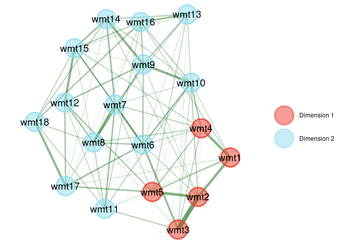
node.label/label.size/label.color
(see Labels below) and
title/legend.title (see Title and Legend below) are also
{EGAnet}-only conveniences, but aren’t shortcuts for a differently-named
ggnet2 argument — they’re just not part of
ggnet2 at all.
Legend
Change Names
plot(ega.wmt, legend.names = c("Dimension 1", "Dimension 2"))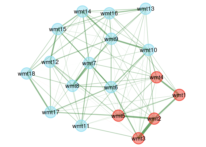
Add a Title
plot(ega.wmt, legend.title = "Community")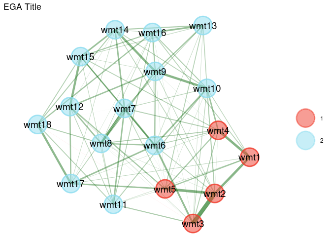
Remove legend
plot(ega.wmt) + theme(legend.position = "none")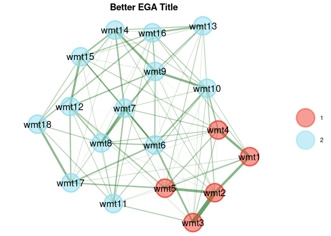
Handling legend title and text can also be done using the standard
?ggplot2::theme arguments, and guides() (below) removes just one legend
at a time rather than all of them.
Title
Basic Title
plot(ega.wmt) + ggtitle("EGA Title")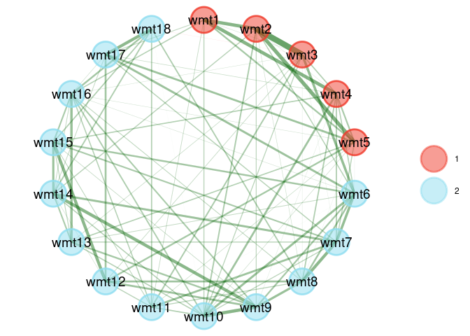
title does the same thing directly, without needing a
separate +:
plot(ega.wmt, title = "EGA Title")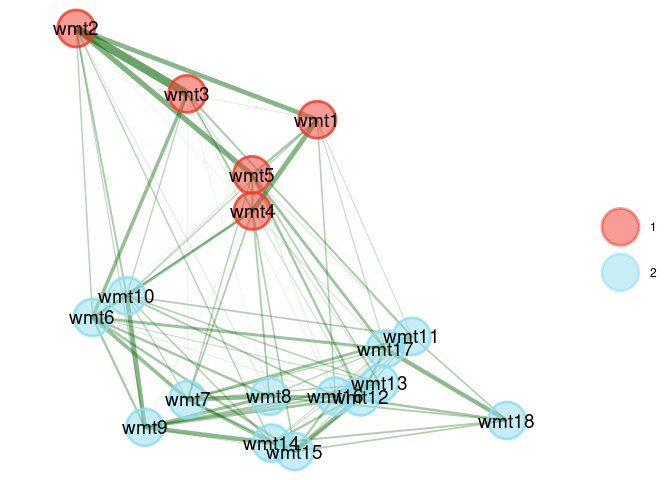
Adjusted Title (centered, larger size, bold)
plot(ega.wmt) +
  ggtitle("Better EGA Title") +
  theme(plot.title = element_text(size = 14, face = "bold", hjust = 0.5))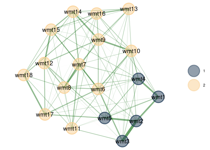
Layout
For all available layout options, see
?sna::gplot.layout. Remove gplot.layout. to
use the layout (e.g., gplot.layout.circle =
layout = "circle")
Circle
plot(ega.wmt, layout = "circle")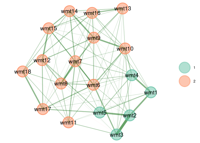
Eigen
plot(ega.wmt, layout = "eigen")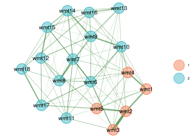
Nodes
Colors
Change Colors Using One of {EGAnet}’s Own Palettes (see
?color_palette_EGA for the full list —
"polychrome", "blue.ridge1",
"blue.ridge2", "rio", "itacare",
"grayscale", and "rainbow")
plot(ega.wmt, color.palette = "blue.ridge2")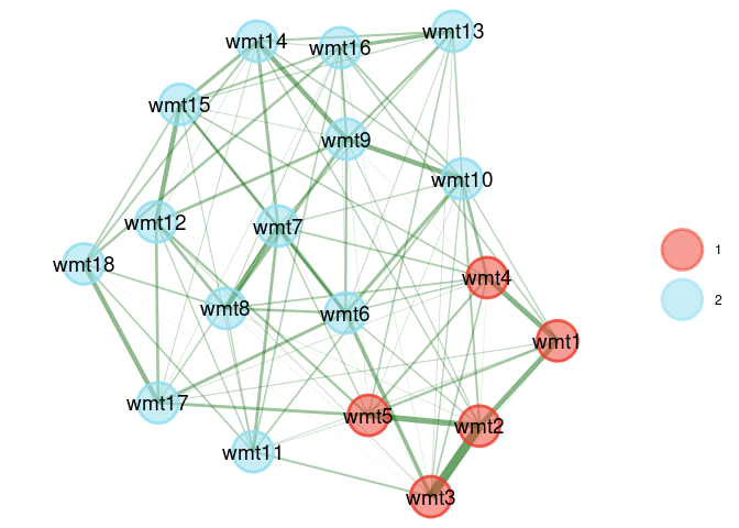
Change Colors Using an {RColorBrewer} Palette (any
palette name from RColorBrewer::brewer.pal.info works)
plot(ega.wmt, color.palette = "Set2")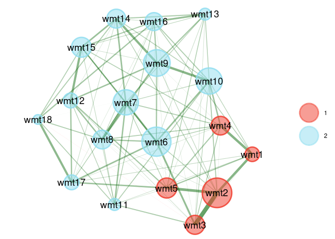
Change Colors Using HEX Codes (one per dimension — handy for matching institutional or journal color schemes)
plot(ega.wmt, node.color = c("#F5815A", "#47BCC9"))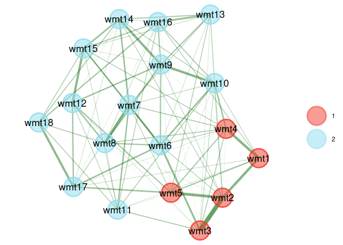
node.color is the one node argument {EGAnet} expands
from “one value per community” to “one value per node” automatically
(it’s what makes the line above work with only 2 hex codes for 18
nodes). Most other node arguments don’t get this treatment — see Sizing and Shaping Nodes
by Community in the advanced section below.
For quick color palette ideas, check out this color palette generator
Size
plot(ega.wmt, node.size = 12)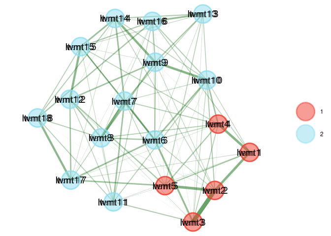
Change Size based on Node Strength
plot(ega.wmt, node.size = colSums(ega.wmt$network)^2 * 16)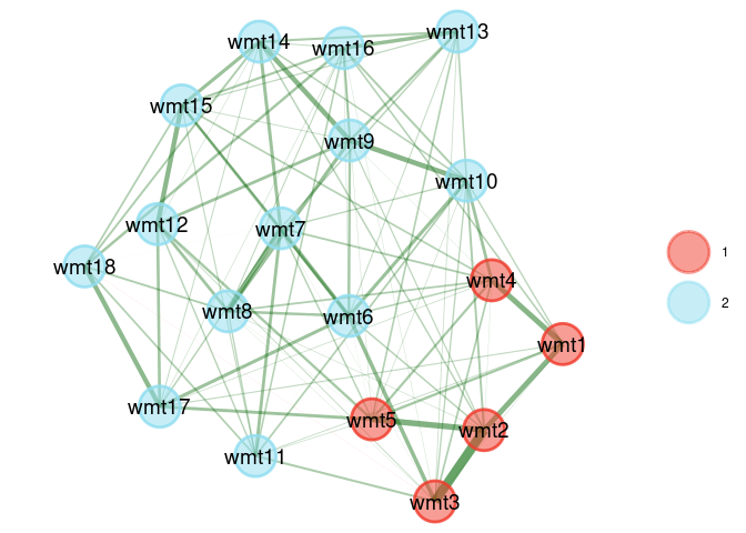
Transparency
plot(ega.wmt, node.alpha = 0.5)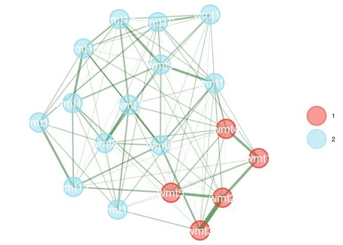
Shape
node.shape takes any base R pch code (see
?graphics::points). The default (19, a solid
circle) is drawn with a matching hollow-circle border; other common
shapes get a matching hollow border too (a square border for
15, a triangle border for 17, and so on):
plot(ega.wmt, node.shape = 17)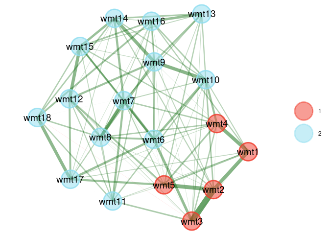
A community-length vector (one shape per community, like
node.color accepts) throws the same kind of error as
node.size does — see Sizing and Shaping Nodes
by Community below.
Labels
Custom Text
By default, nodes are labeled with their column names, but any
character vector of the same length can be used instead — useful for
swapping in full item wording or a different item numbering scheme. Use
node.label for this, not label:
label is left alone on purpose, since composite plots (see
Controlling Panel
Layout of Composite Plots below) also accept
ggarrange’s own labels (plural, for panel
captions) — label vs. labels would be an easy
typo to make and miss, so passing label directly raises a
warning instead of silently doing the wrong thing:
plot(ega.wmt, node.label = paste0("Item ", 1:18))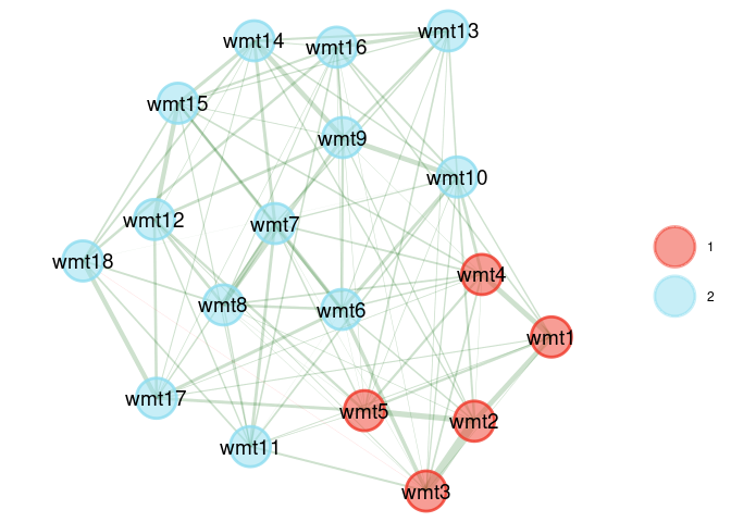
Removing Labels
plot(ega.wmt, label.size = 0)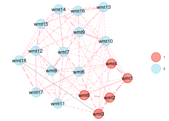
Size and Color
A light label.color (like white) only reads clearly on
top of the node fill, so pair it with a large enough
node.size that the label doesn’t spill past the node’s edge
onto the page background:
plot(ega.wmt, node.size = 18, label.size = 4, label.color = "white")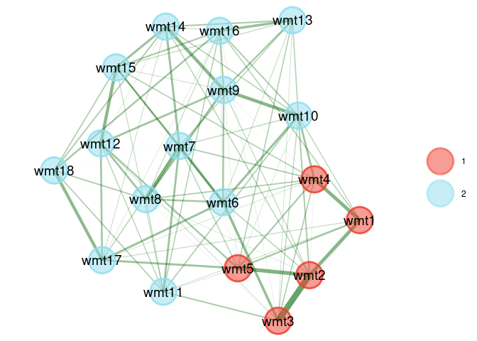
Edges
Size
plot(ega.wmt, edge.size = 12)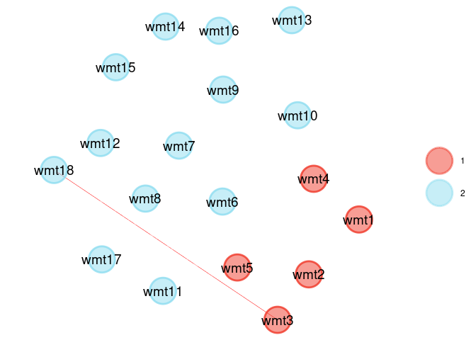
Transparency
plot(ega.wmt, edge.alpha = 0.1)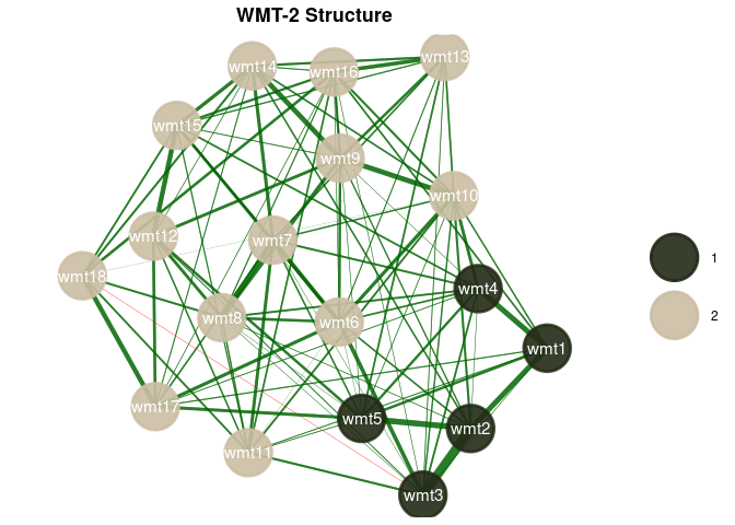
Colors and Line Type
plot(
  ega.wmt, edge.alpha = 1,
  edge.lty = c( # line type
    "dashed", # positive edge first
    "solid" # negative edge second
  ),
  edge.color = c( # color
    "pink", # positive edges first
    "black" # negative edges second
  )
)
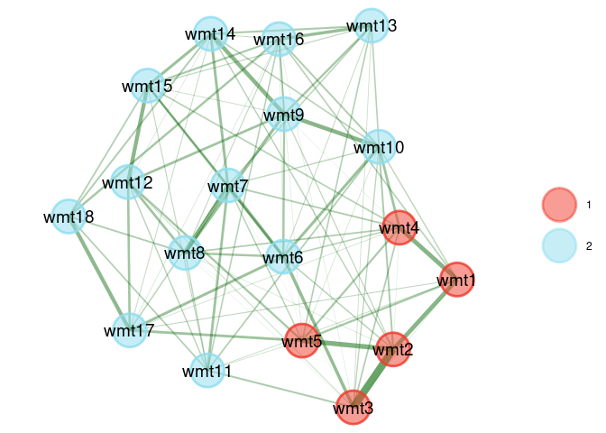
Positive Only
plot(
  ega.wmt,
  edge.color = c(
    "darkgreen", # positive edges (default color)
    "white" # negative edges second
  )
)
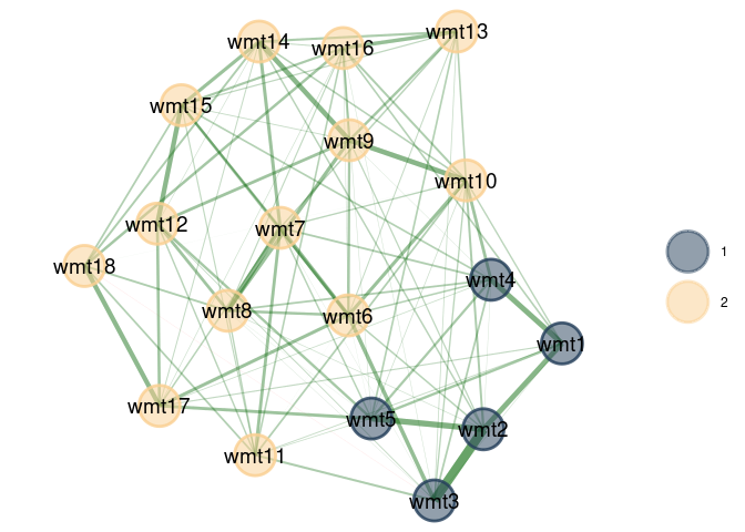
Negative Only
plot(
  ega.wmt, edge.alpha = 1, # used to increase visibility
  edge.color = c(
    "white", # positive edges first
    "red" # negative edges (default color)
  )
)
Edge Value Labels
edge.label is a plain ggnet2 argument (not
something {EGAnet} adds), so it takes a bit more setup than the
shortcuts above — but it’s the way to print the actual network values
(e.g., partial correlations) directly on the edges. Two things
ggnet2 requires that aren’t obvious from the network
alone:
- Length and order.
ggnet2builds its ownnetworkobject from the matrix internally and treats it as directed, so it expects one label per directed edge (bothi -> jandj -> i) rather than one per undirected pair. Rebuilding that samenetworkobject yourself withnetwork::network()and reading it back off withnetwork::as.edgelist()guarantees the labels land in the right order. - No raw negative numbers.
edge.labelerrors on a negative numeric vector – pre-formatting the values as text (sprintf("%.2f", ...)) keeps the minus sign in the label without tripping that check.
This example switches to a smaller, 8-item subset of
wmt2 purely so the labels stay legible — on the full
18-item network above, every edge gets a label and the plot becomes too
dense to read:
ega.small <- EGA(wmt2[,7:14], plot.EGA = FALSE)

# Match `ggnet2`'s internal (directed) edge order
edge_order <- network::as.edgelist(network::network(ega.small$network))
edge_values <- sprintf("%.2f", ega.small$network[edge_order])

plot(
  ega.small, edge.alpha = 0.6,
  edge.label = edge_values, edge.label.size = 3
)
Putting It Together
Every argument above is just one more
ggnet2/ggplot2 layer, so they compose freely
into a single call:
plot(
  ega.wmt,
  color.palette = "itacare",
  node.size = 14, node.alpha = 0.9,
  label.size = 4, label.color = "white",
  edge.alpha = 0.6
) +
  ggtitle("WMT-2 Structure") +
  theme(plot.title = element_text(hjust = 0.5, face = "bold"))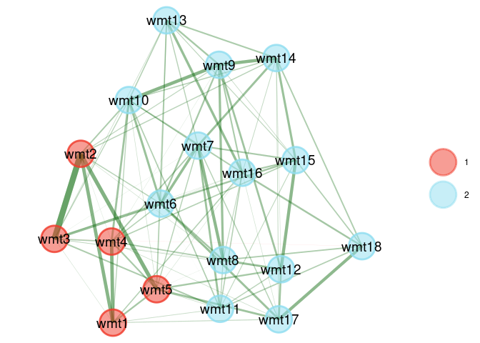
Saving Your Plot
Every plot above is a ggplot2 object, so
ggsave handles exporting it — to PNG, PDF, SVG, or anything
else it supports — at whatever size and resolution you need for a
manuscript or slide deck:
my_plot <- plot(ega.wmt, color.palette = "blue.ridge2")

ggsave("wmt-structure.png", my_plot, width = 6, height = 5, dpi = 300)
Combining with {ggplot2}
Every plot() call above returns an ordinary
ggplot2 object, so anything from {ggplot2}
itself (or an extension package) layers on top with +,
exactly as it would on any other ggplot. The sections above
cover the arguments {EGAnet} and ggnet2 understand
directly; this section covers everything else — themes, annotations,
zooming, and picking apart the legend.
Swapping Themes
{EGAnet}’s default theme hides the axes entirely, since the
coordinates are just a layout, not meaningful units. Swapping in a stock
ggplot2 theme brings some of that back (gridlines, axis
text, and two meaningless axis titles, X1/Y1,
left over from the layout coordinates) — blank those out explicitly
along with the theme:
plot(ega.wmt) +
  theme_minimal(base_size = 13) +
  theme(
    panel.grid = element_blank(), axis.text = element_blank(),
    axis.title = element_blank(), axis.ticks = element_blank()
  )
Aspect Ratio
coord_fixed() controls the ratio of the y- to x-axis
units, useful for stretching a cramped-looking layout or matching a
specific figure aspect ratio for a manuscript:
plot(ega.wmt) + coord_fixed(ratio = 1.4)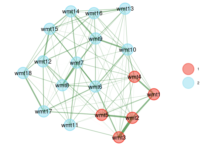
Rich Titles
labs() sets a title, subtitle, and caption together
(title on its own, shown above, only
covers the first):
plot(ega.wmt) +
  labs(title = "WMT-2 Structure", subtitle = "Walktrap algorithm", caption = "N = 1,000")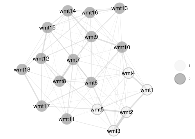
Selective Legends
theme(legend.position = "none") (shown above) removes every legend at once.
guides() targets just one aesthetic — useful once a plot
has more than one legend (e.g., color and size) and only one should
go:
plot(ega.wmt) + guides(color = "none")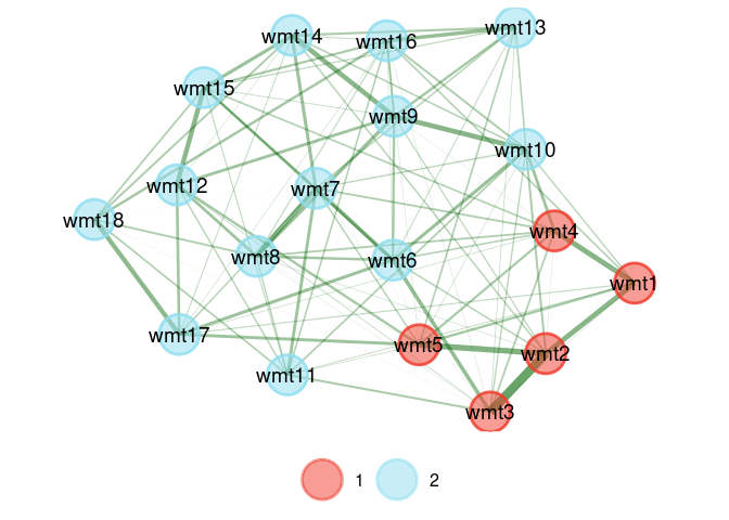
Annotations
annotate() adds arbitrary text, labels, or shapes at
fixed positions. Node/edge coordinates are in the plot’s own (arbitrary)
layout units, which differ from run to run and layout to layout, so
anchoring to the panel edges with -Inf/Inf
(rather than guessing a data coordinate) keeps this robust regardless of
the actual layout:
plot(ega.wmt) +
  annotate(
    "label", x = -Inf, y = -Inf, hjust = -0.05, vjust = -0.5,
    label = "N = 1,000", size = 3.5, fill = "lightyellow"
  )
A Gotcha: Recoloring via
scale_*
A natural instinct coming from other ggplot2 workflows
is to recolor with + scale_color_manual(...) instead of
color.palette/node.color. This doesn’t work
the way it does for a typical ggplot2 plot, and it’s worth
knowing why before it costs debugging time: {EGAnet} draws its nodes
with literal, already-resolved colors (not a mapped color
aesthetic), so a scale_color_manual() added afterward can’t
recolor them. It can still see the legend’s underlying (unused)
color scale, though, and will happily overwrite the legend’s key labels
with whatever values it was given:
# Nodes stay the same colors -- only the legend key labels change,
# to the (otherwise invisible) "purple"/"orange" from `scale_color_manual()`
plot(ega.wmt) + scale_color_manual(values = c("purple", "orange"))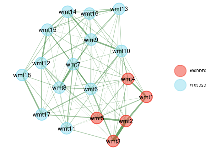
Use color.palette or node.color (see Nodes above) to actually recolor the nodes.
Advanced
The sections below dig into how {EGAnet} builds a plot on top of
ggnet2 under the hood (see
EGAnet:::basic_plot_setup and
EGAnet:::GGally_args in R/plotting.R, if you
want to read the source). Knowing this saves real debugging time — a
couple of arguments look like they should work by analogy with
node.color and quietly don’t.
Every argument passed to a plot.* method is checked
against ggnet2’s arguments, ggarrange’s
arguments (for the composite plots covered below), and
{EGAnet}’s own shortcuts/extras (layout,
alpha, color, shape,
vsize, title, legend.title,
legend.names, arguments). An argument name
that matches none of these — almost always a typo — now throws an
informative error instead of being silently dropped, so a misspelled
edge.colour (British spelling) or nod.size
fails loudly right away instead of quietly rendering with defaults.
Reusing a Layout
Every plot recomputes its node layout from scratch, so plotting the same variables twice — once with each color palette, say — can land the nodes in two different arrangements, which makes the two plots hard to compare side by side.
Passing the hidden arguments = TRUE argument returns the
plot and the exact argument list {EGAnet} handed to
ggnet2, including the node coordinate matrix it computed
(mode):
built <- plot(ega.wmt, arguments = TRUE)

# One row per node, one column per plotting dimension
layout_matrix <- built$ARGS$mode
head(layout_matrix)
[,1] [,2]
[1,] 20.80234 16.56530
[2,] 16.83077 12.80324
[3,] 14.35195 9.68264
[4,] 17.21777 19.35513
[5,] 11.17200 13.27421
[6,] 10.00738 17.79397Feeding that matrix back in as mode locks a second plot
to the same node positions, no matter what else changes:
plot(ega.wmt, mode = layout_matrix, color.palette = "blue.ridge2")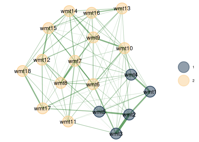
This is exactly what compare.EGA.plots does
internally to keep two structures visually aligned. Saving a layout
matrix by hand is worth doing any time you want multiple figures (in the
same paper, say) to place the same variables in the same spots.
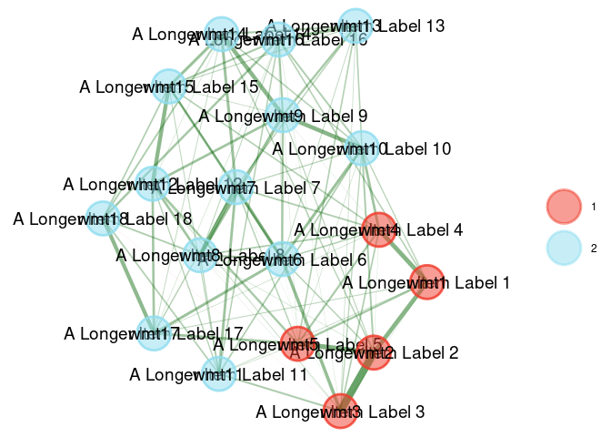
By default there’s also some breathing room built into every plot’s
axes (layout.exp = 0.20) so long node labels don’t get
clipped at the edge. If labels are still clipped — long item wording,
for example — increase it:
plot(ega.wmt, node.label = paste0("A Longer Item Label ", 1:18), layout.exp = 0.45)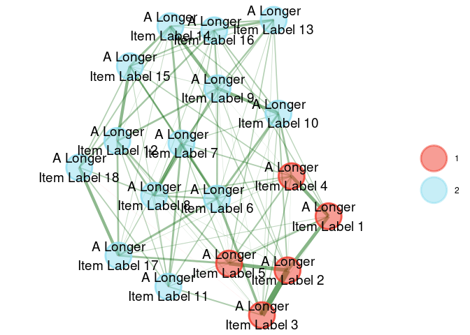
layout.par (arguments passed straight to the underlying
sna::gplot.layout.* function,
e.g. list(niter = 500) to run more Fruchterman-Reingold
iterations) only has an effect once
layout/mode is set to one of
sna’s layouts — {EGAnet}’s default
(mode = "qgraph") uses {qgraph}’s own layout
algorithm and ignores layout.par entirely:
plot(ega.wmt, layout = "fruchtermanreingold", layout.par = list(niter = 500))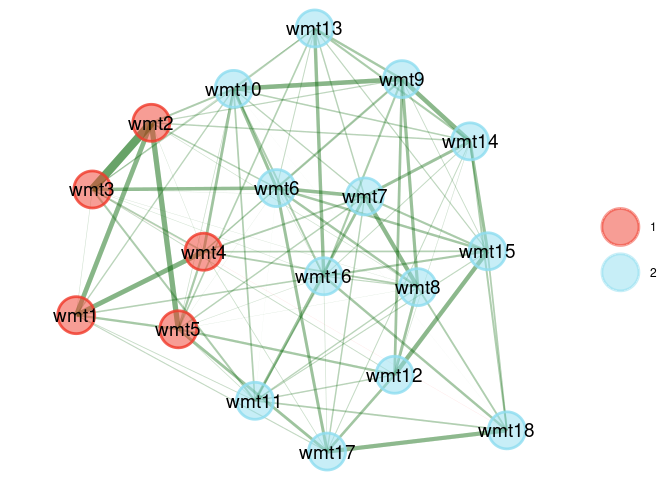
Sizing and Shaping Nodes by Community
As shown in Nodes > Colors above,
node.color accepts one value per community and {EGAnet}
expands it to the full node vector for you. node.size,
node.shape, and node.alpha do
not get the same treatment — a community-length vector
for any of them will build without complaint but throws an error the
moment the plot is actually drawn (printed, knitted, or saved), because
ggnet2 receives a vector that’s neither length 1 nor
length-18:
# This builds without error but fails when it's rendered:
# Aesthetics must be either length 1 or the same as the data (18).
plot(ega.wmt, node.size = c(8, 20))
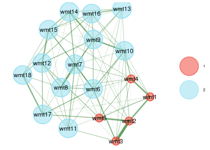
Index by the membership vector yourself to get the per-node vector
ggnet2 expects. This works for node.shape too
— a clean way to distinguish communities by shape as well as color:
plot(ega.wmt, node.size = c(8, 20)[ega.wmt$wc])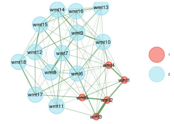
plot(ega.wmt, node.shape = c(19, 17)[ega.wmt$wc])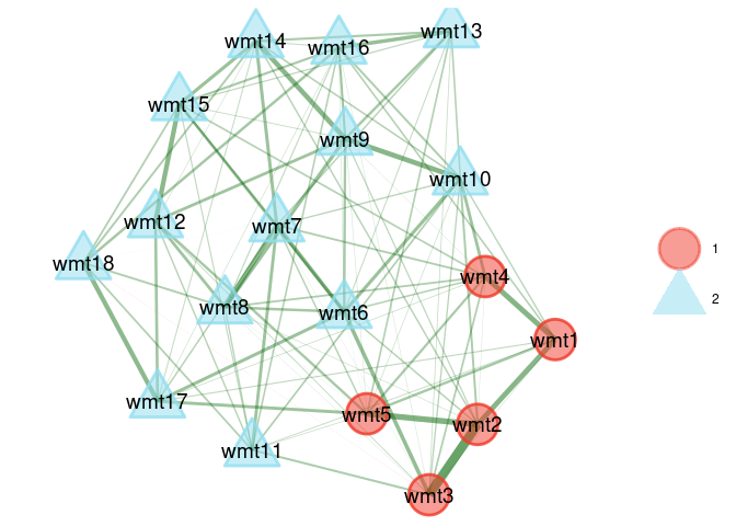
A handful of other ggnet2 arguments are accepted but not
worth reaching for in an {EGAnet} plot:
arrow.size/arrow.type (for directed-graph
arrowheads — {EGAnet} networks are undirected) and
size.cut/size.zero (for continuous
size-aesthetic mapping — {EGAnet} always sets node size directly, per Nodes > Size above) build without error but have no
visible effect. size.min is worth actively avoiding:
setting it currently makes plot() return NULL
with no error or warning at all, rather than a plot.
Accessibility: Colorblind-Safe Plots
color.palette = "colorblind" (an alias for
"grayscale") does more than desaturate the nodes — it also
switches the positive/negative edges to a second, redundant encoding
(solid grey vs. dashed dark grey) so the two edge types stay
distinguishable without relying on color at all:
plot(ega.wmt, color.palette = "colorblind")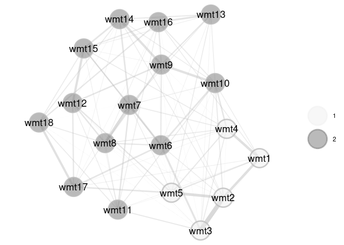
Setting edge.color/edge.lty explicitly (as
in Edges > Colors and Line Type)
overrides this automatic behavior, so it’s an either/or: let
"colorblind" pick a coordinated grayscale + line-type
scheme, or take full manual control.
Legend Position and Size
legend.position and legend.size are plain
ggnet2 arguments that pass straight through, useful when
the default right-hand legend crowds a wide network:
plot(ega.wmt, legend.position = "bottom", legend.size = 12)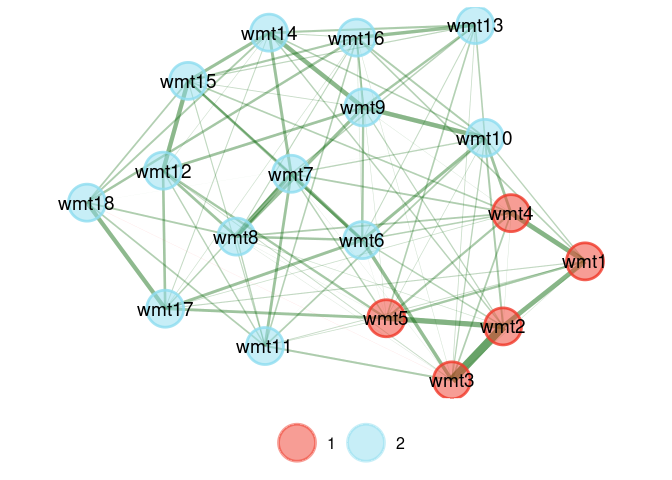
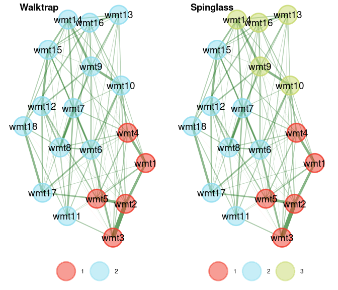
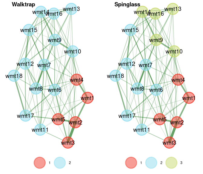
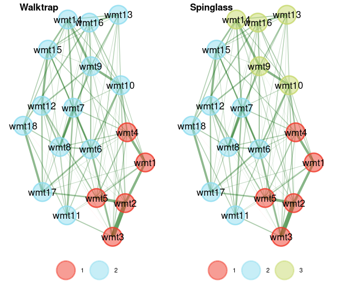
Comparing Structures
compare.EGA.plots (used elsewhere to check bootEGA stability) is itself a
plotting function, and takes the same kind of labeling arguments to keep
multiple structures readable side by side:
ega.wmt.spinglass <- EGA(wmt2[,7:24], algorithm = "spinglass", plot.EGA = FALSE)

comparison <- compare.EGA.plots(
  ega.wmt, ega.wmt.spinglass,
  labels = c("Walktrap", "Spinglass")
)
Controlling Panel Layout of Composite Plots
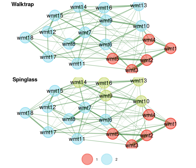
compare.EGA.plots above is a composite plot —
it draws more than one network and arranges them into a single figure
using {ggpubr}’s ggarrange internally. The same is true of
bootEGA, hierEGA (with
plot.type = "separate"), invariance, and
dynEGA.Group/dynEGA.Individual (when plotting
multiple ids). All of these forward unrecognized arguments
to ggarrange in addition to ggnet2, so the
panel layout itself — not just each panel’s styling — can be adjusted
directly from plot():
comparison_stacked <- compare.EGA.plots(
  ega.wmt, ega.wmt.spinglass,
  labels = c("Walktrap", "Spinglass"),
  ncol = 1, nrow = 2, # stack panels vertically instead of side by side
  common.legend = TRUE, legend = "bottom" # share one legend below both panels
)
See ?ggpubr::ggarrange for the full set of layout
arguments (ncol, nrow, legend,
common.legend, align, and more).
Beyond EGA: Other Plot Methods
Every *EGA result plots through the same
ggnet2-based machinery covered above, but a few objects add
their own specialized arguments on top:
| Object | Plot arguments | Full example |
|---|---|---|
hierEGA |
plot.type (“multilevel” or “separate”),
color.match (border lower-order nodes in their higher-order
factor’s color) |
Hierarchical EGA workflow |
invariance |
p_type (“p” or “p_BH”), p_value |
Measurement Invariance workflow |
dynEGA |
base (which plot’s layout to use as the reference),
id (which individual(s) to plot, for
level = "individual") |
Dynamic EGA workflow |
All three still accept every ggnet2 argument from the
sections above (color.palette, node.size,
edge.alpha, and so on) — the arguments in the table just
layer additional structure-specific control on top.