bootEGA — EGAnet

A single EGA result is one estimate from one sample. bootEGA asks how much that estimate would move around if you’d drawn a different sample — generating many bootstrap replicates, re-estimating the network and its communities each time, and summarizing how consistently the original structure reappears. This workflow goes deeper into bootEGA on its own than the full EGA workflow does, including a comparison of its two bootstrap types.

We’ll return to the wmt2 data from the EGA workflow, where the default ("walktrap") empirical solution found two dimensions.

# Load {EGAnet}
library(EGAnet)

# Obtain data
wmt <- wmt2[,7:24]

Parametric vs. Resampling

bootEGA offers two ways to generate bootstrap samples. "parametric" (the default) simulates new datasets from the multivariate normal distribution implied by the estimated network; "resampling" instead draws — with replacement — directly from the rows you actually observed.

boot_parametric <- bootEGA(
  data = wmt, type = "parametric", seed = 1,
  plot.itemStability = FALSE # No plot for CRAN checks
)

summary(boot_parametric)

Model: GLASSO (EBIC)
Correlations: auto
Algorithm:  Walktrap
Unidimensional Method:  Louvain

----

EGA Type: EGA 
Bootstrap Samples: 500 (Parametric)
                                   
                2     3     4     5
Frequency:  0.616 0.344 0.036 0.004

Median dimensions: 2 [0.85, 3.15] 95% CI

boot_resampling <- bootEGA(
  data = wmt, type = "resampling", seed = 1,
  plot.itemStability = FALSE # No plot for CRAN checks
)

summary(boot_resampling)

Model: GLASSO (EBIC)
Correlations: auto
Algorithm:  Walktrap
Unidimensional Method:  Louvain

----

EGA Type: EGA 
Bootstrap Samples: 500 (Resampling)
                                               
                1     2     3     4     5     6
Frequency:  0.004 0.542 0.384 0.066 0.002 0.002

Median dimensions: 2 [0.72, 3.28] 95% CI

Both agree that two dimensions is the most common outcome, and both center their 95% CI on a median of two. But they don’t agree on much beyond that. Parametric bootstrapping puts 61.6% of samples at two dimensions and 34.4% at three, with a comparatively tight CI [0.85, 3.15]. Resampling spreads out more — 54.2% at two dimensions, 38.4% at three, small tails reaching all the way down to one dimension and up to six — and its CI is wider, [0.72, 3.28]. That’s expected: resampling inherits whatever irregularities (skew, outliers, small pockets of missingness) are actually present in your 1185 respondents, while parametric bootstrapping smooths over them by construction. When the two disagree substantially, resampling is usually the more honest picture of what your specific sample can support.

Item Stability

itemStability breaks the same question down by item: of all the bootstrap replicates, what proportion of the time does each item land back in its empirical dimension?

item_stability <- itemStability(boot_parametric)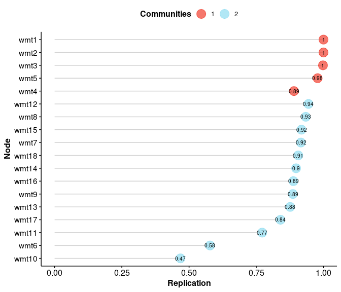

item_stability$item.stability$empirical.dimensions

 wmt1  wmt2  wmt3  wmt4  wmt5  wmt6  wmt7  wmt8  wmt9 wmt10 wmt11 wmt12 wmt13 
1.000 1.000 0.998 0.890 0.978 0.578 0.916 0.934 0.886 0.468 0.772 0.944 0.876 
wmt14 wmt15 wmt16 wmt17 wmt18 
0.898 0.918 0.888 0.840 0.906

Most items replicate well above the 0.70-0.75 range treated as sufficient elsewhere in {EGAnet}. Two don’t: wmt6 (0.578) and wmt10 (0.468). wmt6 is the first item of the empirical second dimension — right at the boundary with the first — so it’s a natural candidate to drift between the two across replicates. wmt10 sits well inside the second dimension, so its instability says something more specific: on its own merits, it doesn’t reliably behave like the rest of that dimension.

Dimension Stability

dimensionStability looks at the same replicates from the dimension’s point of view: not just whether items are individually stable, but whether the entire membership of a dimension reappears identically.

dimension_stability <- dimensionStability(boot_resampling)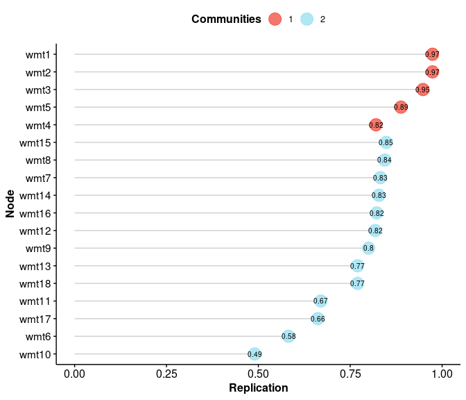

dimension_stability$dimension.stability

$structural.consistency
    1     2 
0.750 0.234 

$average.item.stability
        1         2 
0.9208000 0.7489231

This is where the two summaries pull apart. The first dimension (wmt1-wmt5) has both high average item stability (0.921) and high structural consistency (0.750) — it reappears, intact, in three out of four bootstraps. The second dimension (wmt6-wmt18) has reasonable average item stability (0.749) but low structural consistency (0.234): individually, most of its items are fairly stable, but the dimension rarely comes back with exactly the same 13 items every time. With more items in play, there are simply more ways for one or two of them to shuffle in or out while everything else holds — which is exactly what an exact-match statistic like structural consistency is built to catch, and what an item-by-item stability check alone would miss.

Reproducibility

Every one of those 500 replicates re-estimates a network and re-runs community detection on it — by default, the same Louvain-based check discussed in the EGA workflow, applied 500 times over. Louvain shuffles the order it considers nodes in, so without fixing that randomness up front, the set of 500 bootstrap solutions isn’t guaranteed to reproduce, even on identical data:

# No seed: two runs on the exact same data
boot_noseed_a <- bootEGA(wmt, type = "parametric", plot.itemStability = FALSE, verbose = FALSE)
boot_noseed_b <- bootEGA(wmt, type = "parametric", plot.itemStability = FALSE, verbose = FALSE)

summary(boot_noseed_a)

Model: GLASSO (EBIC)
Correlations: auto
Algorithm:  Walktrap
Unidimensional Method:  Louvain

----

EGA Type: EGA 
Bootstrap Samples: 500 (Parametric)
                                         
                1     2     3     4     5
Frequency:  0.002 0.666 0.294 0.036 0.002

Median dimensions: 2 [0.89, 3.11] 95% CI

summary(boot_noseed_b)

Model: GLASSO (EBIC)
Correlations: auto
Algorithm:  Walktrap
Unidimensional Method:  Louvain

----

EGA Type: EGA 
Bootstrap Samples: 500 (Parametric)
                            
               2     3     4
Frequency:  0.67 0.282 0.048

Median dimensions: 2 [0.87, 3.13] 95% CI

{EGAnet} warns about exactly this when seed is left unset. The two frequency tables above come from identical data and identical settings — the only thing that differed was the random node order bootEGA happened to draw each time. That’s why every call in this workflow has included seed = 1: it fixes that node order (via {EGAnet}’s xoshiro256++ generator, since version 2.5.0) for the whole run, so the same code always produces the same 500 replicates:

# Same seed: two runs on the exact same data
boot_seed_a <- bootEGA(wmt, type = "parametric", seed = 1, plot.itemStability = FALSE, verbose = FALSE)
boot_seed_b <- bootEGA(wmt, type = "parametric", seed = 1, plot.itemStability = FALSE, verbose = FALSE)

identical(boot_seed_a$summary.table, boot_seed_b$summary.table)

[1] TRUE

For a function whose entire purpose is quantifying how stable a structure is, an unreproducible bootstrap would be self-defeating. seed is what makes the stability estimate itself stable.